Dates termed absolute are really of two separate categories. Those, which are stated in terms of years in our calendar, are true absolute dates. The true absolute dates may be derived from tree rings, ancient calendrical systems, coins, and varves where traced directly back in time from present. The other category consists of techniques, which yield dates expressed in years with an associated probability factor. These methods depend on knowing the rate of change and the amount of change, the number of years that have elapsed since the process of change began.
The methods based on this principle are Carbon-14, Potassium-Argon (K-Ar), Uranium-Thorium (Ur/Th), Thermoluminescence (TL), Archaeomagnetic etc.
The term chronometric dating refers to quantitative measurement of time with respect to a given scale. It is synonymous with the more traditional term absolute dating, but is gaining favour among dating specialists who regard it as more appropriate term. The dating methods rely upon the half-life period or the radioactive isotope decay constants are often referred as isotopic dating methods.
(A) Radiocarbon (C 14) Dating
Radiocarbon dating has made a revolutionary impact in the fields of archaeology and quaternary sciences. It is the best known and most widely used of all chronometric dating methods. J. R. Arnold and W. F. Libby (1949) published a paper in Science describing the dating of organic samples from object of known age by their radiocarbon content. Since the radiocarbon dating method became a regular part of the archaeologist’s tool kit we began to have a world chronology for prehistory, based almost entirely on dates obtained by Libby’s technique.
Principles
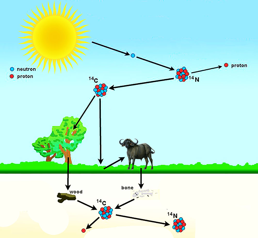
The radiocarbon dating method is based on the fact that cosmic radiation produces neutrons that enter the earth’s atmosphere and react with nitrogen. They produce Carbon 14, a carbon isotope with eight rather than the usual six neutrons in the nucleus. With these additional neutrons, the nucleus is unstable and is subjected to gradual radioactive decay and has a half-life of about 5730 years. Libby’s equation describing the reaction as
N14 = C14 + H1
Chemically C14 seems to behave exactly as ordinary nonradioactive carbon C12 does. Thus the C14 atoms readily mix with the oxygen in the earth’s atmosphere, together with C12, and eventually enter into all living things as part of the normal oxygen-exchange process that involves all living plants and animals. As long as matter is living and hence in exchange with the atmosphere, it continues to receive C14 and C12atoms in a constant proportion. After death the organism is no longer in exchange with the atmosphere and no longer absorbs atoms of contemporary carbon.
After the death of an organism the C14 contained in its physical structure begins to disintegrate at the rate of one half every 5730 years; thus, by measuring the amount of radiocarbon remaining, one can establish the time when the plant or animal died. Half-life (t 1/2) is measured by counting the number of beta radiations emitted per minute (cpm or counts per minutes) per gram of material. Modern C14 emits about 15 cpm/g, whereas C14 5700 years old should emit about 7.5 cpm/g. In the disintegration the C‘14 returns to N14, emitting a beta in the process.
Thus:
C14 = B – + N14 +
Suitable Materials for Radio Carbon Dating
Radiocarbon dates can be taken from samples of many organic materials. The kinds of material selected for C14 dating are normally dictated by what is available. The ideal material for radiocarbon dating is wood and charcoal burned at the time the archeological site was occupied. Bone burned at the time when the site was inhabited can also be dated. Unaltered wood from dry sites, soot, grasses, dung (animal and human), well preserved antler or tusk, paper, calcareous tufa formed by algae, lake mud, parchment, peat and chemically unaltered mollusc shells , Unburned bone contains a substance called collagen, which is rich in carbon, and this can be extracted and dated.
Other vegetable or animal products such as leaves, nuts, paper, parchment, cloth, skin, hide, or hair can be dated but are seldom or never present in prehistoric associations.
Procedure of Radiocarbon Dating
The first stage in the dating procedure is physical examination of the sample. The material is then converted into gas, purified to remove radioactive contaminants, and then piped into a proportional counter. The counter itself is sheltered from background radiation by massive iron shields. The sample is counted at least twice at intervals of about a week. The results of the count are then compared with a modern count sample, and the age of the sample is computed by a formula to produce the radiocarbon date and its statistical limit of error.
A date received from a radiocarbon dating laboratory is in this form: 3,621 ± 180 radiocarbon years before the present (B.P.) The figure 3,621 is the age of the sample (in radiocarbon years) before the present.
With all radiocarbon dates, A.D. 1950 is taken as the present by international agreement. Notice that the sample reads in radiocarbon years, not calendar years.
Corrections must be applied to make this an absolute date. The radiocarbon age has the reading ± 180 attached to it. This is the standard deviation, an estimate of the amount of probable error. The figure 180 years is an estimate of the 360 year range within which the date falls.
The conventional radiocarbon method relies on measurements of a beta-ray decay rate to date the sample. The practical limits of radiocarbon dating with beta decay approaches are between 40,000 to 60,000 years.
Sources of Error in Radio Carbon Dating
Errors of three kinds reduce the absolute dating value of the technique:
(a) statistical-mechanical errors, (b) errors pertaining to the C14 level of the sample itself, and (c) errors related to laboratory storage, preparation, and measurement.
These facts may be outlined briefly.
a) A statistical-mechanical error is present as a result of the random, rather than uniform, disintegration of radioactive carbon. This is expressed in the date by a plus-or-minus value in years (e.g., 6,240±320 yrs.). This statistical error can be reduced by increasing the time of measurement.
b) Sources of error in the C14 content of a sample may be a result of (1) past fluctuations of the C14 concentration in the C14 exchange reservoir; (2) unequal C14 concentration in different materials; and (3) Subsequent contamination of samples in situ.
Archaeological Applications
Radiocarbon dates have been obtained from African hunter-gatherers settlements as long as 50,000 years before the present, from early farming villages in the Near East and the Americas, and from cities and spectacular temples associated with early civilisations. The method can be applied to sites of almost any type where organic materials are found, provided that they date to between about 40,000 years ago and A.D. 1500.
Limitations
Radiocarbon dates can be obtained only from organic materials, which mean that relatively few artifacts can be dated. But associated hearths with abundant charcoal, broken animal bones and burnt wooden structures can be dated. Artifacts contemporary with such phenomena are obviously of the same age as the dated samples. Chronological limits of Carbon 14 dating are accurate from around 40,000 years B.P. to A.D. 1500.
(B) Potassium-Argon (K-Ar) Dating
Next to radiocarbon, the most spectacular results in isotopic dating have been obtained with the potassium-argon method. It is the only viable means of chronometrical dating of the earliest archaeological sites. Geologists use this radioactive counting technique to date rocks as much as 2000 millions years old and as little as 10,000 years old.
Potassium (K) is one of the most abundant elements in the earth’s crust and is present in nearly every mineral. In its natural form, potassium contains a small proportion of radioactive potassium40 atoms. For every hundred potassium 40 atoms that decay, eleven become argon40, an inactive gas that can easily escape from its material by diffusion when lava and other igneous rocks are formed. As volcanic rock forms by crystallisation, the concentration of argon40 drops to almost nothing. But regular and reasonable decay of potassium40 will continue, with a half-life of 1.3 billion years. It is possible, then, to measure with a spectrometer the concentration of argon40 that has accumulated since the rock formed. Because many archaeological sites were occupied during a period when extensive volcanic activity occurred, especially in East Africa, it is possible to date them by associations of lava with human settlements.
A useful cross-check for the internal consistency of K/ Ar dates is provided by paleomagnetic stratigraphy. Unaltered lavas that remain in place undisturbed preserve a record of the earth’s magnetic field at the time of their cooling. Apart from the minor movements of the magnetic poles with time, magnetohydrodynamic processes in the earth’s fluid core have repeatedly reversed the positions of the north and south magnetic poles. Consequently, paleomagnetic data shows a bimodal distribution in “reversed” and “normal” fields. K/Ar dating has demonstrated the existence of normal polarity “epochs” from 690,000 years to the present, and again from 3.3 to 2.4 million years ago, of reversed polarity epochs prior to 3.3 million years and again between 2.4 and 0.69 million years ago. Unfortunately, each of these epochs was interrupted by a number of brief “events,” characterised by rapid switches of the earth’s magnetic field. Although the paleomagnetic record is correspondingly complicated, it nonetheless provides opportunity to check the consistency of K/ Ar dates.
A cross-check on the “absolute” calibration of K/Ar dating has been provided by fission-track dating of volcanic glass from Bed I, Olduvai Gorge. This method uses different assumptions and is prone to other sources of error. The number of “tracks” caused by spontaneous fission of U238 during the “life” of the sample is counted. Age is determined by obtaining the ratio of the density of such tracks to the number of uranium atoms, which is obtained from the increase in track density produced by fission of U235. The Olduvai cross-check provided a fission track age of 2.0 million years that compares reasonably well with K/ Ar dates averaging about 1.8 million years.
Datable Materials and Procedures
Potassium argon dates have been obtained from many igneous minerals, of which the most resistant to later argon diffusion are biotite, muscovite, and sanidine. Microscopic examination of the rock is essential to eliminate the possibility of contamination by recrystallisation and other processes. The samples are processed by crushing the rock, concentrating it, and treating it with hydrofluoric acid to remove any atmospheric argon from the sample. The various gases are then removed from the sample and the argon gas is isolated and subjected to mass spectrographic analysis. The age of the sample is then calculated using the argon 40 and potassium 40 content and a standard formula. The resulting date is quoted with a large standard deviation-J or early Pleistocene site, on the order of a quarter.
Archaeological Applications
Fortunately, many early human settlements in the Old World are found in volcanic areas, where such deposits as lava flows and tuffs are found in profusion. The first archaeological date, and one of the most dramatic, obtained from this method came from Olduvai Gorge, Tanzania, where Louis and Mary Leakey found a long sequence of human culture extending over much of the Lower and Middle Pleistocene, associated with human fossils. Samples from the location where the first cranium of Australopithecus boisei was discovered were dated to about 1.75million years. Even earlier dates have come from the Omo Valley in southern Ethiopia, where American, French, and Kenyan expeditions have investigated extensive Lower Pleistocene deposits long known for their rich fossil beds. Fragmentary australopithecines were found at several localities, but no trace of tools; potassium argon dates gave readings between two and four million years for deposits yielding hominid fossils. Tools were found in levels dated to about two million years. Stone flakes and chopping tools of undoubted human manufacture have come from Koobi Fora in northern Kenya, dated to about 1.85 million years, one of the earliest dates for human artifacts.
Limitations
Potassium-argon dates can be taken only from volcanic rocks, preferably from actual volcanic flows. This laboratory technique is so specialised that only a trained geologist should take the samples in the field. Archaeologically, it is obviously vital that the relationship between the lava being dated and the human settlement, it purports to date be worked out carefully. The standard deviations for potassium-argon dates are so large that greater accuracy is almost impossible to achieve.
Chronological Limits
Potassium argon dating is accurate from the origins of the earth up to about 100,000 years before the present.
(C) PALAEOMAGNETIC OR ARCHAEOMAGNETIC DATING
Introduction
After World War II, geologists developed the paleomagnetic dating technique to measure the movements of the magnetic north pole over geologic time. In the early to mid 1960s, Dr. Robert Dubois introduced this new absolute dating technique to archaeology as archaeomagnetic dating .
The Earth’s magnetic core is generally inclined at an 11 degree angle from the Earth’s axis of rotation. Therefore, the magnetic north pole is at approximately an 11 degree angle from the geographic North Pole. On the earth’s surface, therefore, when the needle of a compass points to north, it is actually pointing to magnetic north, not geographic (true) north . The Earth’s magnetic north pole has changed in orientation (from north to south and south to north), many times over the millions of years. The term that refers to changes in the Earth’s magnetic field in the past is paleomagnetism. In addition to changing in orientation, the magnetic north pole also wanders around the geographic North Pole. Archaeomagnetic dating measures the magnetic polar wander.
Principles
Direction and intensity of the earth’s magnetic field varied throughout prehistoric time. Many clays and clay soils contain magnetic minerals, which when heated to a dull red heat will assume the direction and intensity of the earth’s magnetic field at the moment of heating. Thus if the changes in the earth’s magnetic field have been recorded over centuries, or even millennia, it is possible to date any suitable sample of clay material known to have been heated by correlating the thermoremanent magnetism of the heated clay with records of the earth’s magnetic field. Archaeologists frequently discover structures with well-baked clay floors— ovens, kilns, and iron-smelting furnaces, to name only a few—whose burned clay can be used for archaeomagnetic dating.
Thermoremanent magnetism results from the ferromagnetism of magnetite and hematite, minerals found in significant quantities in most soils. When the soil containing these minerals is heated, the magnetic particles in magnetite and hematite change from a random alignment to one that conforms with that of the earth’s magnetic field. In effect, the heated lump of clay becomes a very weak magnet that can be measured by a parastatic magnetometer. A record of the magnetic declination and dip similar to that of the earth’s actual magnetic field at the time of heating is preserved in the clay lump. The alignment of the magnetic particles fixed by heating is called thermoremanent magnetism.

Datable Materials and Procedures
Substantial floors of well-baked clay are best for the purpose. Tiny pillars of burnt clay that will fit into a brass-framed extraction jig are extracted from the floor. The jig is oriented to present-day north-south and fitted over the pillars, which are then encapsulated in melted dental plaster. The jig and pillar are carefully removed from the floor, and then the other side of the jig is covered with dental plaster as well. The clay sample is placed under suspended magnets and rotated. The scale will record the declination and dip of the remnant magnetism in the clay. An absolute date for the sample can then be obtained if the long-term, secular, variation of the earth’s field for the region is known.
Archaeological Applications and Limitations
From the archaeological point of view, archaeomagnetism has but limited application because systematic records of the secular variation in the earth’s magnetic field have been kept for only a few areas. Declination and dip have been recorded in London for four hundred years, and a very accurate record of variations covers the period from A.D. 1600. France, Germany, Japan, and the southwestern United States have received some attention. At the moment the method is limited, but as local variation curves are recorded from more areas, archaeomagnetism is likely to far more useful for the more recent periods of prehistory, when kilns and other burned-clay features were in use.
Chronological Range
By archaeomagnetic dating one can date two thousand year old human evidence.
(D) DENDROCHRONOLOGY OR TREE-RING DATING
Dendrochronology, or tree-ring dating, was originated in Arisona by A. E. Douglass in about 1913. Tree-ring analysis is a botanical technique with strong analogies to varve study.
Principles
The underlying principle is that nontropical trees add an annual growth increment to their stems. Each tree ring, the concentric circle, representing annual growth, visible on the cross-section of a felled trunk. These rings are formed on all trees but especially where seasonal changes in weather are marked, with either a wet and dry season or a definite alternation of summer and winter temperatures.
Particularly in “stress” zones, along the polar and grassland tree limits, annual radial growth fluctuates widely, depending on the fluctuations of the growing season climate. In warm semiarid regions, available moisture largely controls the rate of radial growth of trees: the tree ring of a moist year is wide, while that of a dry year is narrow or, on occasion, missing entirely. In sub polar regions, rainfall is less significant since the late spring snows keep the water content of the soil sufficiently high. Instead summer, and particularly July, temperatures show the most significant correlation with radial growth.
Dendrochronologists have invented sophisticated methods of correlating rings from different trees so that they build up long sequences of rings from a number of trunks that may extend over many centuries. By using modern trees, whose date of felling is known, they are able to reconstruct accurate dating as far back as 8,200 years. Actual applications to archaeological wood are much harder, but archaeological chronology for the American Southwest now goes back to 322 B.C.

Datable Materials and Procedures
The most common dated tree is the Douglas fir. It has consistent rings that are easy to read and was much used in prehistoric buildings. Pinon and sagebrush are usable, too. Because the latter was commonly used as firewood, its charred remains are of special archaeological interest. The location of the sample tree is important. Trees growing on well-drained, gently sloping soils are best, for their rings display sufficient annual variation to make them more easily datable. The rings of trees in places with permanently abundant water supplies are too regular to be usable. Samples are normally collected by cutting a full cross-section from an old beam no longer in a structure, by using a special core borer to obtain samples from beams still in a building, or by V-cutting exceptionally large logs. Once in the laboratory, the surface of the sample is leveled to a precise plane. Analysing tree rings consists of recording individual ring series and then comparing them against other series. Comparisons can be made by eye or by plotting the rings on a uniform scale so that one series can be compared with another. The series so plotted can then be matched with the master tree-ring chronology for the region. Measuring the tree rings accurately can also add precision to the plottings
Archaeological Applications Absolute Chronology
Extremely accurate chronologies for southwestern sites have been achieved by correlating a master tree-ring sequence from felled trees and dated structures with beams from Indian Pueblos. The beams in many such structures have been used again and again, and thus some are very much older than the houses in which they were most recently used for support. The earliest tree ring obtained from such settlements date to the first century B.C. but most timbers were in use between A. D. 1000 and historic times.
One of the most remarkable applications of tree-ring dating was carried out by Jeffrey Dean (1970), who collected numerous samples from wooden beams at Betatakin, a cliff dwelling in northeastern Arisona dating to A.D. 1270. Dean ended up with no fewer than 292 samples, which he used to reconstruct a history of the cliff dwelling, room by room. Dendrochronology has been used widely in Alaska, the Mississippi Valley, northern Mexico, Canada, Scandinavia, Ireland, the British Isles, Greece, and Germany (Bannister and Robinson, 1975; Baillie, 1982). Recent European research has been especially successful. What the bristlecone pine is to the Southwest, oaks are to Europe.
Arisona tree-ring laboratories are trying to analyse data on annual variability in rainfall from the many trees encompassed by their chronologies. A network of archaeological and modern chronologies provides a basis for reconstructing changing climatic conditions over the past two thousand years. These conditions will be compared with the complex events in southwestern prehistory over the same period.
Limitations
Dendrochronology has traditionally been limited to areas with well-defined seasonal rainfall. Where the climate is generally humid or cold or where trees enjoy a constant water supply, the difference in annual growth rings is either blurred or insignificant. Again, the context in which the archaeological tree-ring sample is found affects the usefulness of the sample. Many house beams have been reused several times, and the outside surface of the log has been trimmed repeatedly. The felling date cannot be established accurately without carefully observing the context and archaeological association of the beam. For this reason, several dates must be obtained from each site. Artifacts found in a structure whose beams are dated do not necessarily belong to the same period, for the house may have been used over several generations.
Chronological Range
Dendrochronology is accurate from approximately seven thousand years ago to the present, with wider application possible. Nonarchaeological tree-ring dates extend back 8,200 years.
(E) Varve Analysis
Varves are annual, graded, bands of sediment laid down in glacier-fed lakes contiguous with the margins of continental glaciers. Detailed work by G. de Geer (1912, and later authors) on such annual sediment layers shows that a new load of sediment enters the lake in the wake of each spring’s thaw. The coarser materials (mainly silts) settle down first while the finer ones (clays) gradually settle during the course of the summer. In larger lakes, wave motion may impede fine sedimentation until autumn when the lake surface freezes over. In numerous cases, fine sedimentation continues under the ice throughout the winter. When coarse silts or fine sands are deposited again during the succeeding spring, a sharp contact zone is formed, so enabling clear identification of the annual increment.
Further seasonal distinctions are provided through biological evidence. The coarse spring time accretion is generally dark and rich in organic matter, while the fine summer sediment is light-colored due to calcium carbonate precipitation. The late summer and autumn sediments are dark again. Pollen examinations of the upper dark layers have shown pollen sequences according to the time of blooming, while microorganisms such as diatoms are concentrated in the light, summer segment.
The thickness of the annual deposit or varve varies from year to year depending on the course of the annual weather and its influence on the ablation of the nearby glacier. A warm year produces large varves, a cold year narrow ones. A requisite to the regular laminar sedimentation is the temperature contrast of warmer, inflowing waters and cold lake waters, whereby the sediment is distributed evenly over the lake bed. Such conditions are best met in ice-margin lakes.
De Geer first recognised that varve sequences were very similar between nearby lakes – within a kilometer of each other – on account of the similarity of local climate. On this basis sequences were correlated and extended in time from area to area. By following the various stands of the retreating ice front. De Geer established an almost complete sequence covering 15,000 years from the late Upper Pleistocene well into historical times. This provided a true chronology whereby glacial features related to the retreat and dissipation of the European glacier could be more or less precisely dated. For example, the close of the Pleistocene was fixed by the event of the draining of the Baltic ice lake, which, according to the varves, occurred in 7912 B. C. Radiocarbon cross-dating suggests that this date may be at most a few centuries off.


Difficulties in the Varve Chronology
Within Fennoscandia the varve-chronology, as established by De Geer (1912, 1940) and Sauramo (1929), has in part remained a respectable body of evidence. It has been shown, however, that storms create multiple varves annually in shallow lakes through addition of extra influx and the stirring of sediments. As most of the lakes south of the Fennoscandian moraines, dating about 9000 B. C., are shallow, the earlier chronology is now considered doubtful.
The establishment of varve-chronologies outside Scandinavia, as attempted by Antevs (1925) in North America, has not been very successful. A major reason for this failure has been extrapolation of sequence segments over hundreds of miles. World-wide correlations of a frivolous type were attempted later whereby reversed seasons in the northern and southern hemispheres, of nonglacial characteristics of varves, have been simply ignored. These attempts have discredited the varve method and generally speaking, other techniques have now replaced the varve chronologies everywhere except in Fennoscandia.
(F) AMINOACID RACEMIZATION (AAR) DATING
All living things use proteins as building blocks in the production of their physical forms. In turn, proteins are composed of folded strands of 20 diverse smaller subunits called “amino acids”. All amino acids, except for one (glycine), come in two different forms known as the laevorotatory (L – left) and dextrorotatory (D – right) form, which are mirror images of each other, but cannot be superimposed one over the other.
What is especially attractive about these two L- and D-forms, at least for the purpose of this topic, is that the vast majority of living things only use the L-form. However, as soon as the creature dies, the L-amino acids start to spontaneously convert into the D-form through a process called “racemization”. If the rate of conversion can be determined, this process of racemization might be useful as a sort of “clock” to determine the time of death.
Basic Assumptions
In order to use the rate of racemization as a clock to exactly estimate when a living thing died, one must know how diverse environmental factors may have affected the rate of change from the L- to the D-form. As it turns out, this rate, which is different for each type of amino acid, is also exquisitely sensitive to certain environmental factors. These include: Temperature; Amino acid composition of the protein; Water concentration in the environment; pH (acidity/ alkalinity) in the environment; Bound state versus free state; Size of the macromolecule, if in a bound state; Specific location in the macromolecule, if in a bound state; Contact with clay surfaces (catalytic effect); Presence of aldehydes, particularly when associated with metal ions; Concentration of buffer compounds; Ionic strength of the environment.
Of these, temperature is generally thought to play the most significant role in determining the rate of racemization since a 1 degree increase in temperature results in a 20-25% increase in the racemization rate (Coote, 1992; Stuart, 1976). Clearly, this factor alone carries with it a huge potential for error. Even slight ranges of error in determining the “temperature history” of a specimen will result in huge “age” calculation errors.
“Amino acid dating cannot obtain the age of the material purely from the data itself. The rate of racemization cannot be standardised by itself because it is too changeable. Thus, because of the rate problem, this dating technique must rely on other dating techniques to standardise its findings. As a matter of fact, the ages obtained from racemization dating must rely on other techniques such as Carbon 14, and if the dating of Carbon 14 is not accurate, racemization dating can never be certain. So, how is it thought to be at all helpful? Well, it is thought to be helpful as a “relative” dating technique.
Interestingly enough, the racemization constant or “k” values for the amino acid dating of various specimens decreases dramatically with the assumed age of the specimens. This means that the rate of racemization was thousands of times (up to 2,000 times) different in the past than it is today. Note that these rate differences include shell specimens, which are supposed to be more reliable than other more “open system” specimens, such as wood and bone.
Add to this the fact that radiocarbon dating is also dependent upon the state of preservation of the specimen. In short, it seems like the claims of some scientists that amino acid racemization dating has been well established as reliable appears to be wishful thinking at best.
Because of these problems AAR dating of bone and teeth (teeth in different locations in the same mouth have been shown to have very different AAR ages) is considered to be an extremely unreliable practice even by mainstream scientists. That is because the porosity of bones makes them more “open” to surrounding environmental influences and leaching. Specimens that are more “closed” to such problems are thought to include mollusk shells and especially ratite (bird) eggshells from the emu and ostrich. Of course, even if these rather thin specimens were actually “closed” systems (more so than even teeth enamel) they would still be quite subject to local temperature variations as well as the other abovementioned potential problems. For example, even today “very little is known about the protein structure in ratite eggshell and differences in primary sequence can alter the rate of Asu formation by two orders of magnitude [100-fold] (Collins, Waite, and van Duin 1999). Goodfriend and Hare (1995) show that Asx racemization in ostrich eggshell, heated at 80 oC has complex kinetics is similar to that seen in land snails (Goodfriend 1992). The extrapolation of high temperature rates to low temperatures is known to be problematic.
(G) OXYGEN ISOTOPE AND CLIMATIC RECONSTRUCTION
Isotopes of a particular environment will have the same chemical properties, but their different masses cause them to be separated or fractioned by certain natural processes.
The oxygen isotopes have been useful in the reconstruction of past environmental condition. It has three isotopes each with a different atomic mass (same number of protons but varying numbers of Neutrons). The oxygen with eight neutrons has an atomic mass of sixteen and is designated 16O, the isotope with nine neutrons is designated 17O, and the isotope with ten neutron is designated 18O. When water evaporates the lighter oxygen isotope (16O) is preferentially incorporated into water vapor, while the heavier isotope (18O) becomes proportionately higher in the remaining water. The fact that 18O is preferentially left in ocean water during evaporation has been used to infer global climatic fluctuations. This has led to a revolution in our understanding of environmental and climatic change during the time of human biological and behavioral development. When this climate change is dated, they can sometimes be used to ascertain the age of archaeological sites. Isotopic signals content in marine sediment, calcite veins and ice core sequence appear to provide a continuous record of global climatic change for the interval associated with the archaeological record. These isotopic signals have been related to relative sea level change and alternative periods of colder global climates (Glacial) and warmer global climates (Inter glacial).
During ice-age the 16O isotope of oxygen does not immediately recycle back into the ocean but instead becomes part of the large ice sheets. The heavy oxygen isotope (18O) becomes more common in oceans during these colder intervals.
This colder isotope ratio is recorded in the shells of Ocean’s living organisms. When warmer global climatic intervals prevail, the lighter isotope, which had been trapped in the ice, returns to the ocean. Thus, during interglacial, there is proportionately less 18O in the oceans. The change in the oxygen isotope ratios have been used to connect artefact bearing deposits with climate chronologies. The variation in oxygen isotopes from the deposits-ridden shell was correlated with the deep sea isotope record. The advantage of the marine oxygen isotope record is that it provides a continuous record of the climatic change that have occurred during the past 2 million years.
URANIUM SERIES DATING
(H) Thorium-Uranium (Ionium-Deficiency) Method
Mollusks, marine coral, and freshwater carbonates contain uranium234 at or shortly after death, but no thorium230 , a daughter element of uranium that is virtually insoluble in natural waters. If the fossil carbonates subsequently remain closed to isotopes of the uranium series, the amount of Th230 present will reflect the original concentration of U234 and the period of isotopic decay. Since the halflife of U234 is 248,000 years, and that of Th230 is 75,000 years, Th grows to equilibrium with U in about 500,000 years. In the meanwhile, the ratio Th230 / U234 is a function of age. The effective dating range of this ionium-deficiency method is 200,000 to 300,000 years.
The major source of error is the introduction of foreign uranium and its daughter products after the death of the organism. To some extent this type of contamination can be screened out, but isolated age determinations cannot be accepted with any great confidence. The Th230/U234 technique has been applied to the study of Pleistocene beaches and lake beds in different parts of the world and there has been sufficient internal consistency as well as consistency with accepted geological correlations to warrant a moderate degree of optimism. In effect, this method has proved crucial for correlating littoral deposits of the last two interglacial periods, both in relation to the radiocarbon-dated portions of the Wurm glacial, and to the apparent temperature fluctuations recorded in organic oozes of the deep-sea floor.
U234 Method
Uranium is present in carbonate solutions in very small concentrations. It is fixed after sedimentation and, barring possible contamination, is not susceptible to outside addition or loss. U234, the daughter element of U238,is originally present in the carbonate solutions but increases through radioactive decay after sedimentation. If the initial proportions of U234 and U238 are known for a particular depositional medium, the U234 / U238 ratio of a fossil carbonate provides an approximate date with a potential dating range of 1 to 1.5 million years (Thurber, 1962). This ratio is fairly constant (1.15) in marine waters but rather variable in fresh waters. Dating of coral has yielded U234 ages consistent with independent age formation, although marine mollusks receive an unpredictable contribution of uranium from surrounding sediments, so that they are less reliable. Dating of freshwater carbonates, such as travertines, has been attempted after establishing the U234 / U238 ratio for modern waters. However, such ratios will vary considerably through time, and the resulting dates are not particularly consistent.
I. Protactinium-Thorium (Protactinium-Ionium) Method
The decay of uranium (U234 and U238 in ocean waters is attended by the formation of daughter elements, Pa231 and Th230 , which accumulate in deep-sea sediments. Being produced by the same element, the ratio of Pa231 (half-life, 32,500 years) and Th230 (half-life, 75,000 years) should be unaffected by the concentration of uranium in marine waters and should be a function of time only, independent of changes in geological conditions. These elements are generally but not always resistant to post-depositional diffusion within the sediment.
Although the laboratory preparation and ultimate analysis of samples is strictly a task for the qualified specialist, it is useful for the persons concerned to be aware of the different results possible, depending on the method of preparation used. There is, at present, no standard method of preparation. Many authors specify their methods, others do not. Some authors have obtained pollen from certain samples by using one technique; others employing another method may fail to find any pollen. Some techniques are widely considered acceptable, while others are frequently considered of dubious validity, other less frequently mentioned but equally serious grievances are directed against over intensive preparation of samples with massive destruction or mutilation of pollen. Since pollen has now been widely and successfully studied from rather “unorthodox,” nonacidic, sedimentary environments in the arid zone and humid tropics, new preparation methods have necessarily been introduced to preserve from wanton destruction.
Until recently the only evaluation of the problem, unfortunately not well suited for the nonspecialist, was a detailed compilation by C. A. Brown (1960). The revised text book of Faegri and Iversen (1964) consequently fills a long-felt need.
Only one, widely employed technique is briefly described here, in order to illustrate the stages of “cleaning.” Three undesirable substances may be present and may be removed in the following manner:
- a) Calcium carbonate is removed with cold, diluted (25 per cent) hydrochloric acid.
- b) Silica is removed by letting the sample stand for 48 hours in 40 per cent concentrated hydrofluoric acid, after which the sample is washed and then heated with 10 per cent hydrochloric acid.
- c) Unwanted organic matter is destroyed by first boiling in 10-15 per cent hydrogen peroxide and then, after washing, boiling the sample a second time in 10 per cent potassium hydroxide.
All three techniques may have to be applied to clays or marls, whereas only (c) may be required in the case of peat, lignite, or coal. When the various undesirables have been so removed, the final residue of pollen is mounted in glycerine jelly on a permanent slide or suspended in liquid glycerine for immediate investigation under the microscope with 300x to 1000x magnification.
J). Thermoluminescence(TL) Method
When a radiation is incident on a material, some of its energy may be absorbed and re-emitted as light of longer wavelength.
The wavelength of the emitted light is characteristic of the luminescent substance and not of the incident radiation.
Thermoluminescence (TL) is the process in which a mineral emits light while it is being heated: it is a stimulated emission process occurring when the thermally excited emission of light follows the previous absorption of energy from radiation. Energy absorbed from ionising radiation (alpha, beta, gamma, cosmic rays) frees electrons to move through the crystal lattice and some are trapped at imperfections in the lattice. Subsequent heating of the crystal can release some of these trapped electrons with an associated emission of light.
If the heating rate is linear and if we suppose the probability of a second trapping to be negligible with respect to the probability of a recombination, the TL intensity is related to the activation energy of the trap level by a known expression. It is so possible to determine the trap depth.
Application on Archaeological findings
Thermoluminescence can be used to date materials containing crystalline minerals to a specific heating event. This is useful for ceramics, as it determines the date of firing, as well as for lava, or even sediments that were exposed to substantial sunlight. These crystalline solids are constantly subjected to ionizing radiation from their environment, which causes some energized electrons to become trapped in defects in the molecular crystal structure. An input of energy, such as heat, is required to free these trapped electrons. The accumulation of trapped electrons, and the gaps left behind in the spaces they vacated, occurs at a measurable rate proportional to the radiation received from a specimen’s immediate environment. When a specimen is reheated, the trapped energy is released in the form of light (thermoluminescence) as the electrons escape. The amount of light produced is a specific and measurable phenomenon.
Material and objects of archaeological or historical interest that can be dated by thermoluminescence analysis are ceramics, brick, hearths, fire pits, kiln and smelter walls, heat treated flint or other heat-processed materials, the residues of industrial activity such as slag, incidentally fire-cracked rocks, and even originally unfired materials such adobe and daub if they had been heated in an accidental fire.
Fundamental principles of dating technique
A non-negligible part of materials which ceramic is usually made of (like quartz and feldspars) is thermoluminescent: those materials have trap states that can capture electrons after interaction with alfa, beta and gamma rays existing in nature.
When these materials are heated to several hundreds of Centigrade degrees, electrons are evicted from trap states and energy is emitted in form of light: thermoluminescence (TL). Heating ceramic in a furnace resets TL accumulated by clay and other materials; from this time on, TL begins growing again as time passes; the more concentrated radioactivity where ceramic is, the quicker TL grows.
Thus by measuring TL we can date an object since the last time it was heated above 400°C. Since measured TL depends on time of exposition to natural radiations but also on the intensity of these radiations, to achieve a precise dating we need information about radioactivity of the area where the object was found.
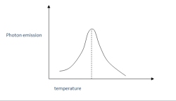
During TL analysis, the sample is reheated by a controlled heating process, so the energy is released in the form of light (thermoluminescence) as the electrons escape. The amount of light produced is measuered by a photomultiplier. The result is a glow curve showing the photon emission in function of the heating temperature:
If the specimen’s sensitivity to ionizing radiation is known, as is the annual influx of radiation experienced by the specimen, the released thermoluminescence can be translated into a specific amount of time since the formation of the crystal structure.
Because this accumulation of trapped electrons begins with the formation of the crystal structure, thermoluminescence can date crystalline materials to their date of formation; for ceramics, this is the moment they are fired. The major source of error in establishing dates from thermoluminescence is a consequence of inaccurate measurements of the radiation acting on a specimen.
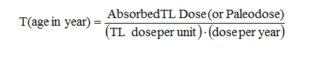
The measure of PALEODOSE
The paleodose is the absorbed dose of natural radiation accumulate by a sample. This paleodose is determined from the TL signal measured by heating sample at a constant rate. The accuracy of the linearity in heating sample is crucial to have a precise measure. The result of this measure is, as described above, a glow curve. Three different types of glow curve can be distinguished:
• The natural thermoluminescence of the sample as it is
• The additive glow curve where a radiation does with a calibrate radioactive source is given in addition to the natural one
• The regenerate signal, when the sample has been zeroed its natural TL by heating and then given an artificial radiation dose
The last two glow curves allow to measure the sensitivity of a sample to natural radiations and are used to determine the paleodose. There are several ways to determine the paleodose comparing the results of the different glow curves measured. The most common methods are:
• The standard method (Aitken, 1985) performs regression analyses for both growth curves and the sum of their absolute values essentially provide the paleodose.
• The normalization method (Valladas & Gillot, 1978; Valladas, 1992; Mercier, 1991), one of the two growth curves is shifted towards the other until they are matched, and the amount of the shift essentially gives paleodose.
The Dose Rate
The denominator Dose rate of the age formula consists of two independent parameters, the internal dose rate and the external dose rate. Obviously, the denominator is crucial for the accurate determination of an age. Internal dose rate all rock material contains radioactive elements that give rise to an internal dose rate. Elements of concern here are only U (Uranium), Th (Thorium), K (Potassium), and to some extent Rb (Rubidium), because other natural radioactive nuclides occur only in very small quantities or do not contribute significantly to the total absorbed dose. Internal dose rate consists of three parameters related to the α, β and γ radiation, where the latter is usually small in most cases. External dose rate sediment contains not only the flint samples, but radioactive nuclides as well. These give rise to an external dose rate in addition to the one from secondary cosmic rays.